Scaling In and Scaling Out: Entry Ladders Explained

At a glance

• Scaling in means filling a planned position size in two or more tranches instead of one order; scaling out means closing it in pieces.
• The average entry is just a size-weighted average of your fills, and it is what your stop and risk must be measured from.
• Tier spacing is usually set by volatility (for example 0.5×ATR) or by structure levels, not by round dollar amounts.
• Laddering improves fill prices in choppy, mean-reverting conditions and hurts in fast trends where the deeper tiers never fill.

Scaling in and scaling out is the practice of entering or exiting a position in several pieces instead of one single order. Instead of buying your whole intended size at one price, you split it into two, three or four tranches placed at different levels; instead of closing everything at one target, you release the position in parts.

Traders care about this because the entry price is one of the few things in a trade you can actually control, and because a position built in tiers behaves differently from a position bought all at once — different average price, different stop distance, different risk, and on perpetual futures, a different liquidation price. Scaling is not an edge by itself. It is an execution technique that changes the shape of your outcomes, and it can just as easily work against you if the tiers are not planned before the trade starts.

What is Scaling In and Scaling Out?

Scaling in is splitting a planned position size across multiple entry orders at different prices. A trader who wants 3 SOL of exposure might place three limit orders of 1 SOL each, spaced below the current price, and accept that only one or two of them may fill.

Scaling out is the mirror image on the exit side: closing one third of the position at a first objective, another third higher, and leaving the remainder to run behind a trailing stop or until a structural level breaks.

Two important distinctions:

• Scaling in ≠ averaging down without a plan. A planned ladder has a fixed total size and a fixed invalidation level decided before the first fill. Averaging down, in the destructive sense, means adding size because the trade is losing, with no size cap and no stop.
• Scaling in ≠ pyramiding. Pyramiding means adding to a position that is already profitable, usually in decreasing size, as the trend extends. Scaling into a pullback adds as price moves against the entry direction, within a predefined zone.

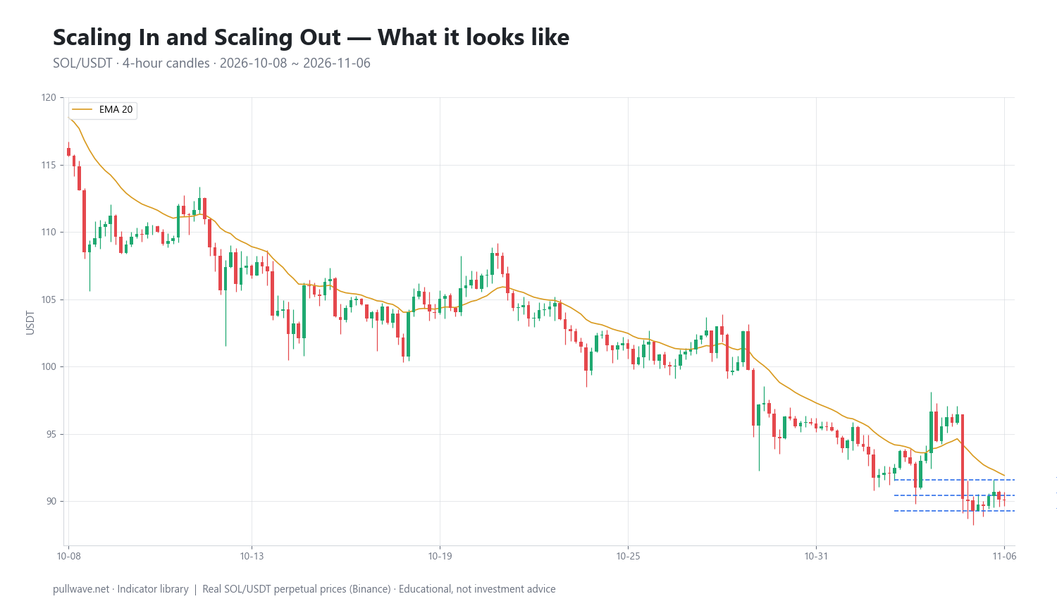
Figure 1 shows the technique drawn on real SOL/USDT 4-hour candles: three horizontal tier lines stacked beneath a pullback area, with the resulting average-entry line sitting in the middle of them. Nothing oscillates and nothing is "triggered" — the ladder is simply a map of where size would be added and where the blended cost basis would end up.

The idea behind it (theory and history)

The idea is older than technical analysis software. Benjamin Graham described formula-based, periodic buying — what later became known as dollar-cost averaging — in The Intelligent Investor (1949), as a way to avoid betting the entire outcome on a single purchase date. The logic is statistical: if you do not know where the low is, spreading purchases across a range guarantees you will not get the worst price, and guarantees you will not get the best one either.

On the trading side, adding to a winning position is strongly associated with Jesse Livermore, whose methods are described in Edwin Lefèvre's Reminiscences of a Stock Operator (1923) and in Livermore's own How to Trade in Stocks (1940). The best-documented modern rule set comes from the Turtle Traders, the group trained by Richard Dennis and William Eckhardt starting in 1983: their published rules added units to an existing position at intervals of 0.5N, where N was a 20-day average true range, up to a maximum of four units, with stops defined in multiples of N. That is the direct ancestor of the volatility-spaced ladders traders use today.

The volatility measure itself, Average True Range, was introduced by J. Welles Wilder Jr. in New Concepts in Technical Trading Systems (1978). Using ATR to space tiers is the key theoretical step: it makes the ladder adapt to the instrument and the moment. A $1.15 gap between tiers is wide on a quiet day and trivially narrow during a liquidation cascade, so spacing is defined in units of current volatility rather than in dollars or fixed percentages.

Van K. Tharp, in Trade Your Way to Financial Freedom (1998), made the broader point that position sizing and exit management — including partial exits — usually affect results more than entry signals do. Scaling belongs to that family of decisions.

How it is calculated

The arithmetic is simple and worth doing by hand once, because most mistakes come from not knowing the blended number.

Step 1 — Fix the total size first. Decide the full position you are willing to hold, based on account risk, before placing any order. The ladder distributes that size; it never increases it.

Step 2 — Choose the anchor. Usually a structure level: a prior swing low, a demand zone, a moving average, a Fibonacci retracement band. The ladder is built around it, with tiers above and below rather than all at one price.

Step 3 — Choose the spacing. Compute ATR over your lookback (14 periods is the common default) on the timeframe you trade, then space the tiers by a fraction of it — 0.5×ATR is the most frequently used increment.

Step 4 — Compute the average entry. It is a size-weighted mean of the fills that actually happened, not of the orders you placed.

Step 5 — Define the stop and the real risk. Risk is measured from the average entry to the invalidation level, multiplied by the size that is actually on.

Step 6 — Plan the exit ladder. Decide in advance what fraction leaves at each objective and what the remainder is managed with.

``` Average entry = Σ(size_i × price_i) / Σ(size_i) Equal tiers = (P1 + P2 + P3) / 3

Tier spacing = k × ATR(n) typical k = 0.5, n = 14 Tier_j = Anchor + (j − 2) × k × ATR(n) (3-tier ladder, j = 1..3)

Risk ($) = |Average entry − Stop| × filled size Average exit = Σ(exit_size_j × exit_price_j) / Σ(exit_size_j) Realized R = (Average exit − Average entry) / (Average entry − Stop) [long] ```

Note the asymmetry hidden in the first formula: a ladder can only ever produce an average better than your highest fill and worse than your lowest fill. It buys you a middle outcome, by construction.

Default settings and variations

Parameter	Common default	Why it exists
Number of tiers	3	Enough to smooth the entry price, few enough to keep fees and tracking manageable
Tier spacing	0.5 × ATR(14)	Scales the ladder to current volatility; inherited from Turtle-style unit adding
Size distribution	Equal (1/3, 1/3, 1/3)	Simplest; average entry equals the arithmetic mean of fills
Stop reference	Average entry, not first fill	Risk must reflect the blended cost basis
Exit ladder	1/3 at first objective, 1/3 at second, 1/3 trailed	Locks partial result while retaining trend exposure

Common variations:

• Weighted ladders. Front-loaded (50/30/20) if you expect a shallow pullback and want most of the size on if the deeper tiers never trade. Back-loaded (20/30/50) if you expect a deep flush and want the bulk of size at the extreme — at the cost of frequently ending up with a small position.
• Wider or narrower spacing. 0.25×ATR keeps tiers tight and raises fill probability; 1.0×ATR spreads them across a much larger zone and often leaves the third tier unfilled.
• Structure-based tiers instead of volatility-based: one at a prior swing, one at a volume-profile node, one at a higher-timeframe moving average. Less mechanical, more context-aware.
• Pyramiding on the exit side reversed: adding in decreasing size only after the position is in profit and the stop has been moved to the average entry.
• Time-based scaling: fixed intervals rather than price levels, closer in spirit to dollar-cost averaging than to trade management.

How to read it

A ladder is read as four numbers, not as a signal: the tier prices, the average if everything fills, the invalidation level, and the resulting dollar risk. If you cannot state all four before the first fill, the ladder is not planned.

The second thing to read is fill probability versus average quality. Tight spacing means almost all tiers fill but the average sits close to your first price — you barely improved anything. Wide spacing means a much better average when the deep tiers fill, but many trades will leave you holding one third of the intended size while price runs away.

The third is what the ladder does to your stop distance. If the invalidation level is fixed by structure, a lower average entry means a tighter stop in percentage terms and therefore a smaller loss if it is hit — but also more size at risk if you filled everything. The two effects partly cancel. Always recompute, never assume.

How traders use it

1. Buying a pullback inside an established uptrend. Tiers are placed through a retracement zone rather than at one guessed price. Works when the market is trending but noisy, and pullbacks routinely overshoot obvious support by a fraction of an ATR. Fails when the trend is so strong that price turns above the first tier — you end up with a third of the intended exposure in your best setup.

2. Accumulating into a range low or a value area. In a sideways regime, where price mean-reverts around a mid-point, laddering across the lower third of the range is a natural fit. Works while the range holds. Fails badly on the range break, which is exactly when all tiers will have filled — so a hard invalidation below the range is non-negotiable.

3. Pyramiding a breakout. Initial size on the break, added units every 0.5×ATR of favorable movement, with the stop raised toward the blended average as units accumulate. Works in sustained directional regimes. Fails in choppy markets, where the added units are bought near local extremes and the whole stack is stopped out on the retest.

4. Scaling out to manage uncertainty. Releasing a third at a measured objective reduces the psychological pressure to abandon the rest, and converts an unrealized number into a realized one. Works when your targets are structural and the market is prone to sharp retracements. Fails in strong trends, where partial exits systematically remove you from the small number of large winners that pay for everything else. There is a real trade-off here: smoother equity curve, lower expectancy per trade.

Example on a real SOL chart

The window below is SOL/USDT perpetual on Binance, 4-hour candles, from 2026-10-08 to 2026-11-06. During this period SOL worked down from a prior high of 116.75 to a pullback low of 89.3 printed on 2026-11-05 20:00 UTC. The last close in the window was 90.1.

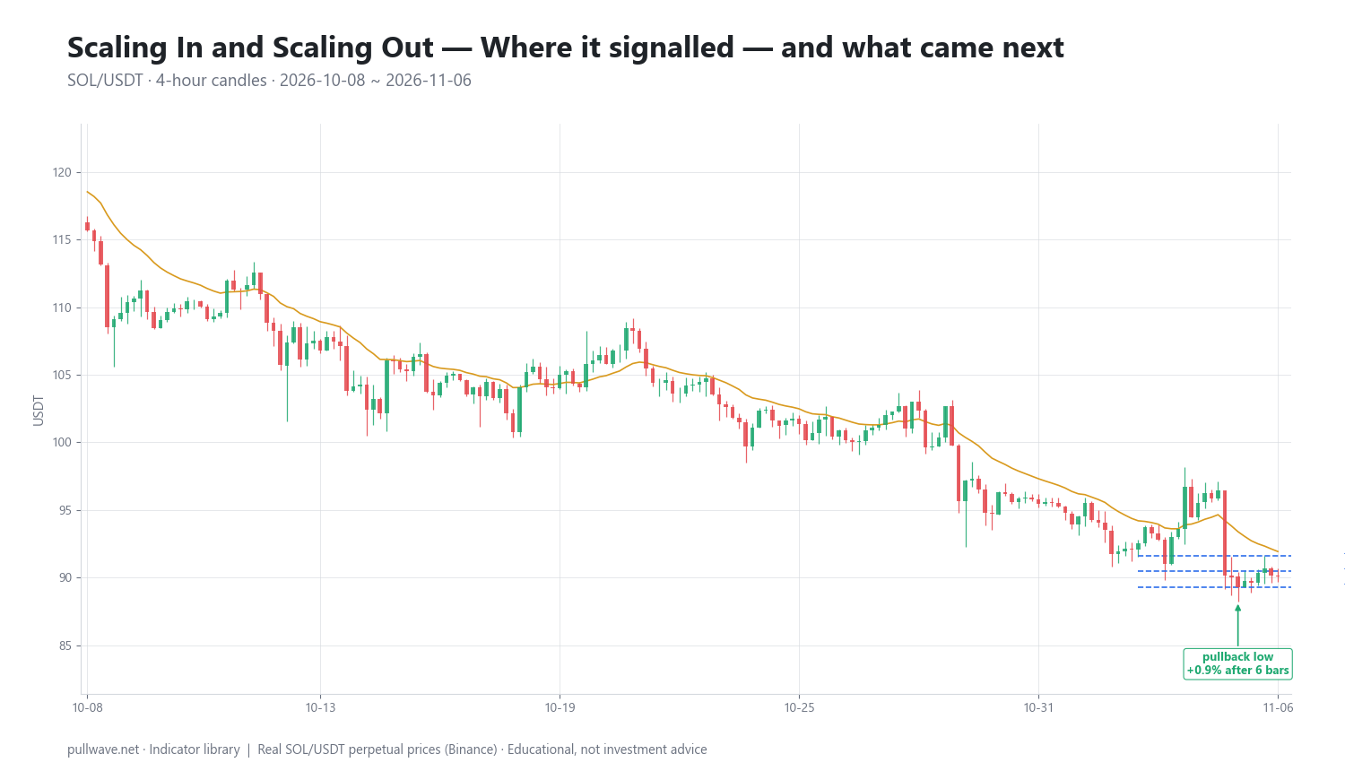
Figure 2 marks the single event recorded in this window — the pullback low at 89.3 — along with the measured move after it. Over the recorded horizon the market moved +0.9% in the direction of the setup. That is 1 of 1 events moving in the signal direction, which is a sample of one and carries no statistical weight whatsoever.

The illustrative ladder uses the settings described above: three equal tiers spaced 0.5×ATR(14) apart around the pullback low, at 91.6 / 90.45 / 89.3. The $1.15 gap between tiers implies an ATR(14) of roughly $2.30 on the 4-hour chart at that time. If all three filled, the average entry would be 90.45, which is 22.5% below the 116.75 prior high.

Now the honest part. At the window's last close of 90.1:

• A single entry at the top tier, 91.6, would be down about 1.6%.
• The three-tier average of 90.45 would be down about 0.4% — still red.
• A single entry exactly at the low, 89.3, would be up 0.9%.

The ladder did what a ladder does: it produced a middle outcome. It avoided the worst fill and missed the best one. It did not make the trade profitable within this window, and it did not predict the low — the deepest tier filled only because price happened to reach the level that was later identified as the low.

For completeness, a hypothetical invalidation one ATR below the low would sit near 87.00, giving roughly $3.45 of risk per unit from the 90.45 average, about 3.8%. That number, not the entry price, is what determines how much size the account can carry. One illustration on one market over one month tells you nothing about how the technique performs in general; it only shows the arithmetic in context.

Common mistakes

• No total size cap. If each new tier is decided in the moment, you are not scaling — you are adding to a loser with an open-ended budget. The total must be fixed before the first fill.
• Measuring risk from the first fill. Risk is always measured from the blended average with the size actually on. Traders who track only their first entry consistently underestimate exposure.
• Moving the stop down as tiers fill. The invalidation level comes from market structure. If filling a lower tier makes you want to lower the stop, the stop was in the wrong place or the thesis has changed.
• Treating a half-filled ladder as a full position. If only the first tier filled, you have one third of the planned size. Profit targets and expectations should scale accordingly.
• Over-fragmenting. Eight tiers on a small account means eight sets of fees, eight partial fills, and a cost basis you cannot recall under pressure.
• Scaling out of everything, every time. Systematically taking partials in a trending regime caps the right tail. Decide in advance which regime you are in and whether a trailing stop would serve better.
• Ignoring funding and holding costs. On perpetual futures, a position held in pieces across days accrues funding on the full notional that is open at each settlement, commonly every eight hours.

Crypto-specific considerations

Crypto markets run 24/7, which means a resting ladder will fill while you sleep, including during thin weekend liquidity when a single large order can sweep several tiers at once. Long lower wicks are common on perpetual markets during liquidation cascades, so the deepest tier may fill on a wick that reverses within minutes — occasionally an excellent fill, occasionally the first leg of a far larger move.

On leveraged perpetuals the critical point is that each added tier moves your liquidation price. Adding size at lower prices on a long raises the liquidation level toward the market, even as it improves the average entry. Under cross margin the whole account balance buffers the position; under isolated margin only the assigned margin does. Recomputing the liquidation price after every fill, and keeping the stop meaningfully inside it, is the difference between a managed ladder and a countdown.

Timeframe matters for spacing. On a 4-hour chart, 0.5×ATR(14) might be about a dollar on SOL near $90; on a 5-minute chart the same formula produces tiers so close together that fees dominate. Match the ladder's width to the timeframe that defines your invalidation.

Combining it with other tools

• ATR supplies the spacing and the stop distance, keeping both in the same volatility units.
• Support and demand zones, or volume profile nodes, give the ladder an anchor with a reason behind it rather than an arbitrary price.
• Fibonacci retracement bands are widely used to place tiers across the 0.5–0.786 region of a prior leg, with invalidation beyond the origin of the move.
• Anchored VWAP from a swing low or a major event provides a dynamic anchor that many participants watch.
• Momentum oscillators such as RSI, especially divergence at the deepest tier, can act as confirmation that selling pressure is fading — never as a reason to override the size cap.
• A higher-timeframe trend filter (for example a 200-period moving average on the daily) tells you whether you should be laddering into pullbacks at all, or whether the regime favors a single entry on strength.

The common thread: every one of these tools answers where and whether, while scaling answers how much, at which prices. Keep the two decisions separate.

Frequently asked questions

Q. What is the difference between scaling in and averaging down?

Scaling in is a planned distribution of a fixed total size across predefined price levels, with a stop decided before the first fill. Averaging down, in its harmful form, is adding unplanned size to a losing position in the hope of recovering the loss, with no size cap and no invalidation. The orders can look identical on a chart; the difference is entirely in whether the total size and stop existed before the trade began.

Q. How many tiers should I use when scaling into a crypto position?

Two to four is the usual practical range, with three being the most common compromise. Fewer tiers mean less fee drag and a cost basis you can remember; more tiers smooth the average but fragment the position and complicate management. On smaller accounts, fees and minimum order sizes often make more than three tiers counterproductive.

Q. Does scaling in reduce risk?

Not by itself. Risk is total size multiplied by the distance from the average entry to the stop, and a ladder changes the average entry, not the size cap or the invalidation level. What scaling does reduce is timing risk — the chance that your entire position sits at the single worst price in a volatile zone. If the ladder is used as an excuse to hold more size than planned, it increases risk.

Q. Should I scale out of a winning trade or use a trailing stop?

It depends on the regime you believe you are in. Scaling out realizes part of the gain and lowers variance, which suits range-bound or mean-reverting markets where retracements are deep and frequent. A trailing stop keeps full size in the trade and captures more of the rare large trends, at the cost of giving back more on every reversal. Many traders blend the two: a partial exit at a structural objective, the remainder trailed.

Q. How does scaling into a perpetual futures position affect liquidation price?

Every added tier increases notional exposure and shifts the liquidation price closer to the market, even though the average entry improves. On a long, adding at lower prices raises the liquidation level; on a short, adding at higher prices lowers it. Recalculate after each fill, and treat a stop placed comfortably inside the liquidation level as part of the plan rather than an afterthought.

Q. Is dollar-cost averaging the same as scaling into a trade?

They share the arithmetic but not the purpose. Dollar-cost averaging is time-based, open-ended, and typically used for long-horizon accumulation without a stop. Scaling into a trade is price-based, size-capped, and tied to a specific invalidation level that ends the position if the thesis fails.

Key takeaways

• Scaling in distributes a fixed total size across predefined price tiers; the total and the invalidation level must exist before the first fill.
• Your average entry is a size-weighted mean of actual fills, and every risk calculation — stop distance, dollar risk, liquidation buffer — must be recomputed from it.
• Volatility-based spacing such as 0.5×ATR(14) adapts the ladder to the instrument and the moment, which fixed dollar gaps cannot do.
• Laddering tends to help in choppy or mean-reverting conditions and to leave you underweight in strong trends; scaling out does the reverse, smoothing results while capping the largest winners.
• In the SOL illustration, a three-tier ladder at 91.6 / 90.45 / 89.3 produced a 90.45 average that was still slightly underwater at the 90.1 close, even though price rose 0.9% off the 89.3 low — a middle outcome, from a single observation that proves nothing about the technique in general.

---

Educational material. Charts use real SOL/USDT perpetual prices; past behaviour does not predict future results. Not investment advice.