Indicator & technique library · Trading techniques

Mean Reversion Strategy Explained: Formula and Settings

Q: Does mean reversion work in crypto?

Mean reversion appears in crypto the same way it appears in other markets: price spends most of its time inside a two-sigma envelope and often snaps back after short, sharp excursions. But crypto's leverage-driven liquidation cascades and 24/7 trading produce deeper and faster overshoots than most traditional markets, so position sizing and stops matter more than signal quality. It is a regime-dependent technique, not a constant property of the market.

Q: What is the best indicator for a mean reversion strategy?

There is no single best one. Standard-deviation bands (20-period, 2σ) and the equivalent z-score are the most direct measurement because they adapt to volatility; Keltner channels using ATR are a smoother alternative; short-period RSI is popular for pullback entries. What separates results is the regime filter and the risk rule attached to the indicator, not the indicator itself.

Q: What timeframe is best for mean reversion trading?

Intraday-to-swing timeframes such as 1h and 4h are the most common compromise in crypto: enough observations to be statistically meaningful, enough movement to cover fees and funding. Lower timeframes generate many signals but the average excursion shrinks toward transaction costs. The right choice is the timeframe where the measured half-life of deviations fits your intended holding period.

Q: How do I know if a market is ranging or trending before I fade it?

Look at the slope of the mean and at how price behaves at the bands. A flat or gently oscillating 20-period average with single closes outside each band is range behavior; a sloped average with consecutive closes hugging one band is trend behavior. A longer-term average, ADX, or a simple higher-high/higher-low structure check gives the same answer with fewer judgment calls.

Q: Is mean reversion better than trend following?

Neither dominates; they have opposite return profiles. Mean reversion wins often with small gains and occasional large losses, trend following loses often with small losses and occasional large gains. They tend to perform well in different regimes, which is why some traders run both rather than choosing.

Q: What does the half-life of mean reversion mean?

Half-life is the estimated number of bars it takes for a deviation from the mean to shrink by half, derived from fitting an Ornstein–Uhlenbeck-style regression to the series. It gives you an objective basis for the holding period and time stop of a reversion trade. If the half-life is long relative to your intended hold, the trade is closer to a directional bet than a statistical one.

Updated 2026-11-04

At a glance

Mean reversion is the assumption that price tends to return toward a statistical average after stretching away from it.
The standard measurement is a moving average plus standard-deviation bands, or the equivalent z-score of price.
It performs best in balanced, range-bound regimes and fails badly during trending or liquidation-driven moves.
In a 4h SOL/USDT window from 2026-10-05 to 2026-11-03, 88.3% of closes stayed inside 20/2 bands and 11 of 13 band closes moved in the fade direction over the shorter outcome horizon, while most longer-horizon outcomes went the other way.

Mean reversion is not an indicator — it is an assumption about how a market behaves. The assumption is simple: when price stretches unusually far from some average, the distance tends to shrink again, either because price comes back or because the average catches up. Almost every oscillator, band and channel on a chart is a way of measuring that distance.

Traders care about it because it is the natural counterpart to trend following. Trend strategies win by holding through continuation and lose many small trades; mean reversion strategies win often and lose rarely but badly. Knowing which regime you are in — and how to measure "unusually far" with numbers instead of eyesight — is most of the work.

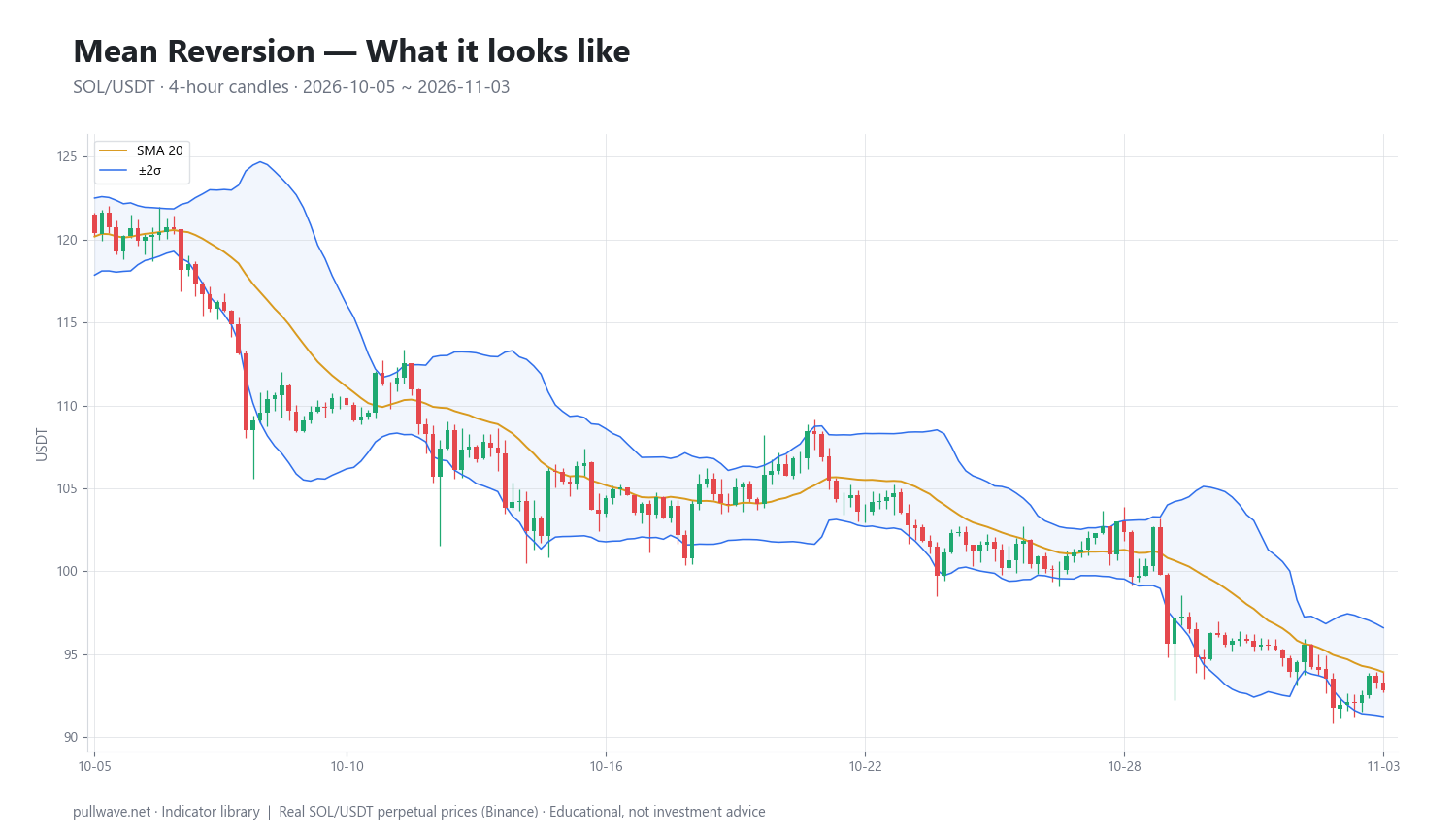
Mean Reversion Strategy Explained: Formula and Settings — 1

Figure 1 shows the measurement applied to real SOL/USDT 4h candles: a 20-period simple moving average with bands at two standard deviations above and below. The band width breathes with volatility, and price spends most of its time inside the envelope.

What is Mean Reversion?

Mean reversion is the tendency of a series to pull back toward a central value after a deviation. In trading, the "mean" is usually a moving average of price (20-period SMA, VWAP, an anchored average) and the deviation is measured in standard deviations or in multiples of average true range.

Important distinction: a mean-reverting series is not the same as a falling series. Price can revert toward a mean that is itself sliding downward. A long signal taken because price is 2.5 standard deviations below a 20-period average can be "correct" — the gap closes — while the position still loses money, because the mean fell to meet price instead of price rising to meet the mean.

Mean reversion can also be measured on things other than raw price: the spread between two correlated assets (pairs trading), funding rates on perpetual futures, basis between spot and futures, or an oscillator such as RSI. The logic is identical in each case — define a normal level, measure the excursion, trade the shrinkage.

The idea behind it (theory and history)

The statistical root is older than markets. Francis Galton described "regression towards mediocrity" in his 1886 paper on hereditary stature, showing that extreme measurements in one generation are followed by less extreme measurements in the next. The mathematical workhorse is the Ornstein–Uhlenbeck process, introduced in 1930 to describe a velocity that is continuously pulled back toward an equilibrium level — still the standard model for a mean-reverting price spread.

In finance, the empirical case was built in the 1980s. De Bondt and Thaler's 1985 paper Does the Stock Market Overreact? documented long-horizon reversal in US equities, and Poterba and Summers (1988) and Lo and MacKinlay (1988) debated how much of short-horizon price movement is predictable rather than a random walk. At roughly the same time, quantitative desks on Wall Street began trading the spread between correlated stocks — statistical arbitrage — which is mean reversion applied to a relationship rather than to a single price.

On the chart side, the tools arrived separately. Chester Keltner described a moving-average channel in How to Make Money in Commodities (1960). Welles Wilder published RSI in New Concepts in Technical Trading Systems (1978). John Bollinger developed standard-deviation bands in the early 1980s, explicitly to make the envelope adapt to volatility instead of using a fixed percentage.

Why should price revert at all? Three economic reasons are usually offered: liquidity providers demand a premium to absorb one-sided order flow and then unwind it; forced sellers and forced buyers (margin calls, liquidations, redemptions) push price past where informed participants think value is; and crowd reaction to news overshoots the information content. None of these guarantee reversion — they just make it common enough to measure.

How it is calculated

The most common quantitative form is the z-score of price against a moving average, which is exactly what standard-deviation bands draw. Step by step, for a 20-period lookback:

Take the last 20 closes.
Average them. That is the mean (the 20-period SMA).
For each of the 20 closes, subtract the mean and square the result.
Average those squared differences and take the square root. That is the standard deviation (population form, dividing by 20, is the convention used by charting packages).
Upper band = mean + 2 × standard deviation. Lower band = mean − 2 × standard deviation.
The z-score of the current close = (close − mean) ÷ standard deviation. A close exactly on the upper band has z = +2.

SMA20 = sum(close[i], i=1..20) / 20 sigma = sqrt( sum((close[i] - SMA20)^2, i=1..20) / 20 ) upper = SMA20 + 2 * sigma lower = SMA20 - 2 * sigma z = (close - SMA20) / sigma %b = (close - lower) / (upper - lower)

Two extra numbers are worth computing if you trade this seriously. Band width = (upper − lower) ÷ SMA20 tells you whether volatility is expanding or contracting. Half-life estimates how long a deviation takes to decay by half: regress the one-bar change of the series on its previous level, Δy_t = α + β·y_{t−1} + ε, then half-life = −ln(2) ÷ ln(1 + β). If the half-life on your timeframe is 200 bars, a 6-bar fade has no statistical basis.

half_life = -ln(2) / ln(1 + beta) # beta from dy_t = alpha + beta*y_(t-1)

Default settings and variations

The 20-period, 2-standard-deviation default comes from Bollinger: 20 trading days is roughly a calendar month, and two standard deviations would capture about 95% of observations if returns were normally distributed. They are not normal — they have fat tails — so in practice something closer to 85–90% of closes land inside the bands. The SOL window measured below came in at 88.3%, which is typical.

Variation	Typical setting	What changes
Standard bands	20 SMA, 2σ	Balanced default; ~85–90% of closes inside
Tight bands	20 SMA, 1.5σ	More signals, more false fades, smaller edge per signal
Wide bands	20 SMA, 2.5–3σ	Rare signals, deeper excursions, longer waits
Keltner channel	20 EMA, 2 × ATR(20)	Uses range instead of close dispersion; smoother, fewer squeezes
Short-term RSI	RSI(2) or RSI(3)	Popularized by Larry Connors for equity pullbacks; very reactive
VWAP bands	Session/anchored VWAP ± σ	Volume-weighted mean, useful for intraday crypto

Shorter lookbacks (10) react faster and make the mean follow price so closely that deviations rarely look extreme. Longer lookbacks (50, 100) define a slower equilibrium and produce fewer but larger excursions. Use an EMA instead of an SMA if you want the mean to weight recent price more heavily; it reduces lag but makes the band calculation less statistically clean.

How to read it

Read three things, in this order:

Slope of the mean. Flat or gently waving means a balanced market where fades have a reasonable base rate. Steeply sloped means a trend, and fades against it are counter-trend trades, whatever the z-score says.
Band width. Narrow and contracting often precedes expansion; wide and expanding usually means something real is happening and the first touch of a band is not an exhaustion signal.
Position and persistence. One close outside a band is an excursion. Several consecutive closes outside the same band — "walking the band" — is the signature of a trend, not of overextension.

A z-score above +2 does not mean expensive. It means statistically unusual relative to the last 20 bars. In a market that has just repriced on news, unusual is exactly what you should expect.

How traders use it

1. Range fades. In a sideways market, a close beyond a band with a flat mean is used as a signal to lean the other way, with a target near the mean and an invalidation beyond the recent extreme. Works when volatility is stable and there is no fresh catalyst. Fails the moment the range breaks; the first trending leg typically produces several losing fades in a row.

2. Pullback entries inside a trend. Instead of fading the extreme, the trader fades with the trend: in an uptrend, a touch of the lower band or an oversold oscillator is treated as a discount entry toward the rising mean. Works because it combines two edges — reversion plus trend. Fails when the pullback is the start of the reversal, which is why a structural stop below the prior swing matters more than the band itself.

3. Spread and relationship reversion. Trading the deviation between two correlated assets, between perpetual and spot, or in funding rates — crowded positioning tends to normalize. Works when the relationship is economically anchored. Fails when the correlation structure breaks (a chain halt, a listing, a depeg), which is precisely when the spread looks most attractive.

4. Volatility targeting rather than direction. Some traders use band width and z-score only to size positions — smaller when the market is stretched and volatile, larger when it is quiet — without taking a directional reversion trade at all. This is the lowest-risk use of the concept and the one that fails least often.

In crypto, two specifics change the math. Markets run 24/7, so there are no gaps to absorb overnight information — excursions develop inside continuous price action, often during thin weekend liquidity. And on perpetual futures, leverage turns an orderly deviation into a cascade: liquidations force market orders in the direction of the move, which extends the excursion far past where a two-sigma band sits. A mean-reversion trade with no stop and 10x leverage is a position that can be liquidated while the thesis is still technically correct.

Example on a real SOL chart

The window is SOL/USDT perpetual on Binance, 4h candles, from 2026-10-05 to 2026-11-03, using a 20-period SMA with bands at 2 population standard deviations. Over that window 88.3% of closes finished inside the bands — close to the long-run figure for a two-sigma envelope on a fat-tailed series — and the last close was 92.81. There were 13 closes outside a band. Outcomes are measured 6 bars (one day) and 18 bars (three days) later.

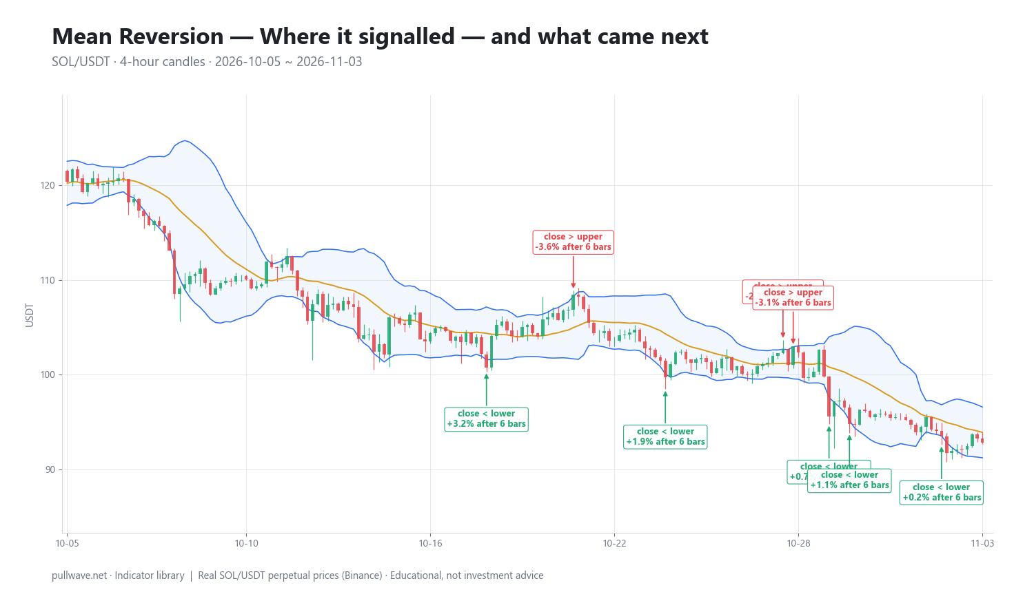
Mean Reversion Strategy Explained: Formula and Settings — 2

Figure 2 marks each signal on the same chart with its subsequent percentage move. Across all 13 band closes, 11 of 13 had moved in the direction of the fade after the shorter horizon. That sounds encouraging until you look at the two horizons side by side.

Date (UTC)	Signal	Price	After 6 bars	After 18 bars
2026-10-12 20:00	close < lower	105.70	+1.02%	−0.30%
2026-10-14 12:00	close < lower	103.82	+2.14%	−0.25%
2026-10-18 16:00	close < lower	100.78	+3.19%	+7.41%
2026-10-21 12:00	close > upper	108.44	−3.56%	−8.04%
2026-10-24 12:00	close < lower	99.72	+1.88%	+1.20%
2026-10-28 08:00	close > upper	102.71	−2.31%	−6.70%
2026-10-28 16:00	close > upper	103.02	−3.15%	−7.03%
2026-10-29 20:00	close < lower	95.62	+0.71%	−1.16%
2026-10-30 12:00	close < lower	94.81	+1.15%	−1.38%
2026-11-02 12:00	close < lower	93.50	+0.24%	−0.74%

The pattern in this particular window is instructive. Every lower-band close shown produced a positive 6-bar move, but most of those bounces were small — +0.24%, +0.71%, +1.15% — and by 18 bars, five of the seven had turned negative. The market was drifting lower throughout: price went from the 105 area in mid-October to a 92.81 close on 3 November. The mean kept falling, so buying two sigma below it bought a bounce, not a bottom.

The three upper-band closes behaved differently. Each one was followed by a decline at both horizons, and the declines grew with time: −3.56% then −8.04% from 108.44, −2.31% then −6.70%, −3.15% then −7.03%. Those are the signals that happened to point the same way as the prevailing drift.

Treat this as one illustration on one market over one month, not as evidence that the technique works. Thirteen observations prove nothing statistically, and the results were genuinely mixed: good hit rate on the short horizon, poor outcomes on the long horizon for every fade that leaned against the direction of the market. A different asset or a different month could easily reverse the picture.

Common mistakes

Fading a trend because the z-score is extreme. The most expensive mistake in this family. In a strong move, price can close outside the band for many bars in a row while the band itself migrates.
No stop, or a stop based on the band. Bands widen as volatility rises, so a stop placed "just outside the band" moves away from you exactly when you need it. Use structure or a fixed multiple of ATR.
Confusing frequent wins with profitability. Mean reversion naturally produces high hit rates and small average wins. One ungoverned loss can erase twenty of them. Track expectancy, not win rate.
Ignoring the half-life. If deviations on your timeframe decay over days, a six-bar holding period is a coin flip. Measure the decay rate before choosing a target and a time stop.
Averaging down with leverage. Adding to a losing reversion trade on perpetual futures is how an acceptable loss becomes a liquidation. The position size at which you would be comfortable being wrong twice more is the size to start with.
Over-optimizing the band multiple. Finding that 2.3σ beat 2.0σ on last quarter's data is almost always curve fitting.

Combining it with other tools

The single most valuable companion is a regime filter. A long-period moving average slope, ADX, or a simple comparison of current band width to its own average will tell you whether to fade extremes or to only take reversion entries in the direction of the larger trend. Many traders simply refuse counter-trend fades when the 100- or 200-period average is clearly sloped.

Volume and order-flow context helps separate exhaustion from initiation. A band excursion on collapsing volume often reflects thin liquidity; the same excursion on record volume with a wide range usually signals new information. Divergence between price and an oscillator such as RSI or MACD adds a second, independent reading of momentum loss.

Horizontal structure matters more than the band. A lower-band close that lands on a level where the market previously traded heavily is a different proposition from one in the middle of empty space. In crypto, funding rates add a sentiment layer: deeply negative funding alongside a lower-band excursion suggests crowded shorts, while persistently positive funding during an upper-band excursion suggests crowded longs.

Finally, pair the measurement with an explicit time stop. If the deviation has not decayed within roughly one half-life, the reason for the trade has expired even if the stop has not been hit.

Frequently asked questions

Q. Does mean reversion work in crypto?