Grid Trading Explained: Formula, Settings and Uses

At a glance

• Grid trading places a ladder of orders across a chosen price range and pairs each fill with an opposite order one step away.
• The step is simply the range divided by the number of intervals: (high − low) / (levels − 1), or a constant ratio for geometric grids.
• It harvests oscillation inside a range and bleeds when price trends away, because the ladder keeps accumulating inventory against the move.
• On SOL/USDT 4h (2026-10-07 to 2026-11-05), a 9-line grid from 88.24 to 103.89 gave a 1.96 step and 61 level touches in 60 bars.

Grid trading is not an indicator that tells you where price is going. It is an order-placement technique: you divide a price range into evenly spaced lines, place buy orders below the market and sell orders above it, and let each fill be closed by an opposite order one step away. The profit comes from price oscillating through the ladder, not from a correct forecast.

Traders care about it because it turns volatility itself into a source of realized gains, and because it is mechanical — once the range, the number of lines and the size per line are set, there is nothing to decide bar by bar. The cost of that simplicity is that a grid has a built-in bias toward holding whatever the market is selling: it buys all the way down and sells all the way up. Understanding exactly where that cost appears is the whole subject of this page.

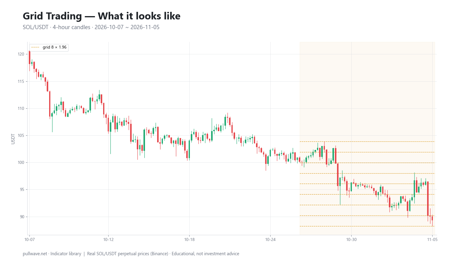
Figure 1 shows the technique drawn on real SOL/USDT 4-hour candles: nine horizontal lines spanning the high and low of the most recent 60 bars, with the candles weaving through them. What matters visually is not the lines themselves but how often price crosses them and whether the range holds at the edges.

What is Grid Trading?

A grid is a set of price levels, equally spaced in price (arithmetic) or in percentage (geometric), covering a range you define. Each level carries a resting order. Levels below the current price are buys; levels above are sells. When a buy fills, the system places a sell one step higher; when a sell fills, it places a buy one step lower.

The technique has three variants. A neutral grid keeps roughly balanced exposure and trades both directions, usually on futures. A long grid only buys dips and sells them back, accumulating spot inventory when price falls. A short grid is the mirror image and only exists on margin or derivatives.

What a grid actually measures is nothing — it is an execution framework. Its edge, if any, comes from a hypothesis you supply: that price will keep oscillating inside the chosen range long enough for the round trips to outpay fees, funding and the inventory loss at the boundaries.

The idea behind it (theory and history)

Grid trading has no single documented inventor. The mechanics are much older than the retail name: they are a simplified version of what dealers and market makers have always done — quote on both sides of a reference price and earn the spread while carrying inventory risk. The academic treatment of that trade-off dates to Amihud and Mendelson's 1980 dealership model and Ho and Stoll's 1981 work on optimal dealer pricing under inventory and return uncertainty, and was formalized for electronic order books by Avellaneda and Stoikov in 2008.

A second theoretical root is rebalancing. The idea that systematically trimming a volatile asset against cash can extract value from oscillation even when the asset goes nowhere is usually associated with Claude Shannon, who described such a scheme in a lecture in the 1960s; the account most people cite is William Poundstone's retelling in Fortune's Formula (2005). The effect is sometimes called volatility pumping. A grid is essentially a rebalancing rule expressed as resting limit orders instead of periodic adjustments.

The retail term "grid trading" spread through foreign-exchange communities in the 2000s, often bundled with martingale position sizing, before being adopted wholesale by crypto traders in the late 2010s when exchanges began offering built-in grid order types. Claims about a specific originator should be treated skeptically — the technique was reinvented many times.

The honest theoretical statement is this: a grid converts path-dependent oscillation into realized cash flow, and finances that cash flow by accepting a growing position against any sustained move. It is short volatility in direction and long volatility in path.

How it is calculated

Step by step:

1. Choose the range. Pick a lower bound and an upper bound. Common choices: the low and high of the last N bars, a visually obvious support/resistance band, or price ± a multiple of ATR.
2. Choose the number of lines. With n lines there are n − 1 intervals between them.
3. Compute the step. For an arithmetic grid, divide the range by the number of intervals. For a geometric grid, take the (n − 1)-th root of the high-to-low ratio.
4. Place the levels. Each level is the low plus i steps (or the low times the ratio to the power i).
5. Assign sides. Levels below current price get buy orders, levels above get sell orders.
6. Set size per level. Usually total capital divided by the number of buy levels, so the ladder can be fully filled without margin stress.
7. Define the pairing rule. Each fill is matched with an opposite order exactly one step away.

``` Arithmetic grid range = high - low step = (high - low) / (levels - 1) L_i = low + i * step for i = 0 .. levels-1

Geometric grid r = (high / low)^(1 / (levels - 1)) L_i = low * r^i for i = 0 .. levels-1

Gross per round trip (arithmetic) profit = step * size_per_level Net net = profit - entry_fee - exit_fee - funding_cost (perps) ```

With the SOL/USDT settings used in Figure 1: high 103.89, low 88.24, 9 lines. The range is 15.65, divided by 8 intervals, giving a step of 1.96 (1.95625 before rounding). The nine levels fall at roughly 88.24, 90.20, 92.15, 94.11, 96.07, 98.02, 99.98, 101.93 and 103.89.

Note the step as a percentage: 1.96 on a price near 96 is about 2.0%, but the same 1.96 near 88 is about 2.2%. That asymmetry is exactly why geometric grids exist on assets with wide ranges.

Default settings and variations

There is no canonical default. These are the parameters that actually change behavior:

Parameter	Common choice	Why it exists
Range source	High/low of last 30–100 bars	Recent range is the cheapest estimate of where price has been willing to oscillate
Number of lines	5–20	More lines = more fills, smaller profit each, higher fee drag
Spacing	Arithmetic (narrow ranges), geometric (wide ranges)	Geometric keeps every round trip the same percentage
Step size	0.5× to 1.5× ATR of the working timeframe	Ties spacing to actual bar-to-bar movement instead of a round number
Mode	Long-only, neutral, short	Determines inventory risk direction
Boundary rule	Stop, pause, or re-center outside the range	Without one, the grid has no invalidation

The 60-bar lookback used in the example is a middle-of-the-road choice: long enough that one spike does not define the range, short enough that the grid tracks the current regime. Shorter lookbacks re-center quickly but whipsaw; longer ones give wide, stable grids with few fills.

On step size, the binding constraint is cost. If your round-trip fee plus expected funding is 0.1% and your step is 0.3%, one third of the gross profit is gone before slippage. A useful sanity check: step should be at least five to ten times the all-in round-trip cost.

How to read it

Read three things off a grid chart.

Where price sits in the ladder. In the example the last close is 89.3, sitting in the lowest cell between 88.24 and 90.20 — roughly half a step above the floor. For a long grid built on that range, this is the state where almost every buy level has already filled and almost the entire ladder is unsold inventory. The position is near maximum long, right at the point where the range is most likely to break.

How often price crosses the lines. Over the 60 bars used to build the grid, the nine lines were touched 61 times — an average of about one touch per bar. That density is what a grid needs. A grid drawn on a window with a handful of touches is a grid that will sit idle or get run over.

Whether the edges are holding. A grid is only as good as its boundaries. If price is repeatedly tagging the top line and closing above it, the range hypothesis is failing regardless of how many fills have accumulated.

How traders use it

1. Range harvesting in sideways markets. The classic use: define a consolidation, lay a grid across it, collect the oscillation. Works when a market has clear horizontal boundaries and high intrabar movement — common in crypto during post-trend digestion phases. Fails the moment the range resolves; the grid is fully loaded on the wrong side exactly when the breakout happens.

2. Laddered accumulation on spot. Instead of a single entry, a trader places a long-only grid below price to average into a position, and lets the sell side scale out on bounces. Works for a trader who actually wants the asset and has reserved the full capital for every level. Fails when the ladder is sized as if all levels will never fill — which is the one scenario that guarantees they will.

3. Neutral grids on perpetual futures. A balanced grid that trades both sides with leverage, aiming to be roughly delta-neutral at the center. Works in choppy, high-volatility conditions where funding is near flat. Fails badly under leverage: the liquidation price is a hard boundary the grid does not know about, and a one-sided funding regime can quietly outcost the round trips.

4. Distribution ladders. A holder places sell levels above price to exit a position in slices rather than all at once. Works as a discipline tool, removing the single-decision problem. Fails as a profit engine in strong uptrends, where it sells the position long before the move ends.

Example on a real SOL chart

The illustration uses SOL/USDT perpetual on Binance, 4-hour candles, from 2026-10-07 to 2026-11-05. The grid was constructed from the high and low of the most recent 60 bars: low 88.24, high 103.89, nine lines, giving a step of 1.96. The last close in the window was 89.3.

The interesting statistic is the touch count: across those 60 bars the nine grid lines registered 61 touches. On average that is one level interaction per bar, which is the kind of density a grid is designed for — price was moving through roughly 2% increments repeatedly rather than parking between lines.

The second observation is positional. With price finishing at 89.3, in the lowest cell of a range whose top is 103.89, a long grid built on this window would have been carrying close to a full inventory load. That is the structural feature worth internalizing: high touch counts and maximum drawdown in inventory tend to arrive together, because a market that oscillates its way lower is both filling your buys and marking them down.

The study logged no discrete entry events over this window under the rule set being tested, so the planned 6-bar and 18-bar follow-through measurements produced nothing to report. That is a real result, not an omission: with zero qualifying events, this window says nothing about whether the technique's signals lead anywhere. It only shows the geometry and the interaction frequency.

Treat all of this as one illustration on one market over one 30-day window. It does not demonstrate that grid trading works, and it is not a backtest. A different lookback, a different step, or the same settings one month earlier would produce different numbers.

Common mistakes

• No invalidation. A grid without a rule for what happens outside the range is an unhedged position with extra steps. Decide in advance whether you stop, pause, or re-center.
• Sizing for the average case. Allocating as if only half the buy levels will fill means the other half fill on margin. Size for every level filling.
• Martingale add-ons. Doubling size at each lower level turns a bounded loss into an unbounded one. The historical association between grids and martingale is the main reason the technique has a poor reputation.
• Ignoring funding on perps. A grid that holds a persistent long into a positive-funding regime pays every eight hours, and that cost is invisible in the fill log.
• Steps too tight for the fee schedule. Hundreds of fills can still net a loss if each round trip barely clears costs.
• Fitting the range to a trending window. If the last 60 bars were a clean trend, their high and low define a channel the market has already left.
• Reading fill count as performance. Fills are activity, not profit. Unrealized inventory loss does not appear in the fill count.

Combining it with other tools

The decision a grid cannot make for you is should there be a grid here at all. That is a regime question, so pair it with regime tools.

Trend strength filters. ADX, a choppiness index, or a simple comparison of close-to-close movement versus the high-low range help classify whether the market is oscillating or directional. Many traders only deploy a grid when the trend reading is weak.

ATR for geometry. Use ATR on the working timeframe to set both the step (so spacing matches typical bar movement) and the range width, instead of picking round numbers.

Volatility bands. Bollinger Bands or Keltner Channels give an adaptive estimate of where the range edges are. A Bollinger squeeze is a warning, not an invitation: compression usually precedes the expansion that breaks a grid.

Volume profile. The value area of a profile is a more structurally meaningful range than a rolling high-low, because it marks where volume actually transacted.

Higher-timeframe structure. A 4-hour grid inside a daily downtrend is a mean-reversion bet against the dominant timeframe. Knowing that does not forbid the trade, but it should change the size.

Funding rate. On perpetuals, persistent funding is a direct carry cost or credit on grid inventory and belongs in the expected-value calculation alongside fees.

Frequently asked questions

Q. What is grid trading in crypto?

Grid trading is a technique that divides a chosen price range into evenly spaced levels and places buy orders below the current price and sell orders above it. Each filled buy is paired with a sell one step higher, so the strategy realizes small profits as price oscillates. It is popular in crypto because markets trade 24/7 and often spend long stretches ranging with high intrabar volatility.

Q. Does grid trading work in a trending market?

Structurally, no — a grid is a mean-reversion framework. In a sustained trend the ladder keeps filling on the losing side and accumulates inventory against the move, while the opposite side goes untouched. Some traders use one-sided grids aligned with the trend direction, but a standard range grid in a strong trend is the scenario where it performs worst.

Q. How many grid levels and what spacing should I use?

There is no universal answer, but the practical constraint is cost: each round trip must clear fees, funding and slippage with room to spare. A common approach is to set the step at roughly 0.5 to 1.5 times the ATR of your working timeframe, then let the number of levels follow from the range width. In the SOL example, a 15.65-wide range with 9 lines produced a 1.96 step, about 2% per round trip.

Q. What is the difference between an arithmetic and a geometric grid?

An arithmetic grid uses a constant price step, so every level is the same dollar distance apart. A geometric grid uses a constant ratio, so every level is the same percentage apart. Geometric spacing is generally preferred on wide ranges or volatile assets, because it keeps the profit per round trip consistent in percentage terms across the whole ladder.

Q. Is grid trading safe with leverage?

Leverage does not change the logic of a grid but it changes the consequences of being wrong about the range. A grid loads up exactly as price moves against it, so the position is largest when it is furthest offside — which is precisely when a leveraged account approaches liquidation. Any leveraged grid needs its liquidation price calculated for the fully filled case before the first order is placed.

Q. How do funding rates affect a grid on perpetual futures?

A grid that carries net long or short inventory pays or receives funding at each settlement, typically every eight hours. In a market with persistently positive funding, a long-biased grid pays a continuous carry cost that is separate from fees and can exceed the realized grid profit during slow periods. Checking the prevailing funding regime is as important as checking the range.

Key takeaways

• A grid is an execution framework, not a forecast: the step is just (high − low) / (levels − 1), and all the edge or loss comes from whether the range assumption holds.
• It profits from path — oscillation through the lines — and loses from direction, because the ladder always accumulates inventory against a sustained move.
• The parameters that matter are the range source, the step relative to ATR and to trading costs, the size per level assuming full fill, and an explicit rule for what happens outside the boundaries.
• In the SOL/USDT 4h window shown, nine lines from 88.24 to 103.89 gave a 1.96 step and 61 level touches in 60 bars, with price closing at 89.3 near the floor — a single illustration of both the fill density and the inventory risk, not evidence of profitability.
• Leverage, funding and martingale sizing are the three additions that most often turn a bounded grid loss into an account-level one.

---

Educational material. Charts use real SOL/USDT perpetual prices; past behaviour does not predict future results. Not investment advice.