Dollar-Cost Averaging (DCA) in Crypto: Formula and Uses

At a glance

• Dollar-cost averaging means investing a fixed amount of money at fixed intervals, regardless of price.
• Because the fixed amount buys more units when price is low, the resulting average cost is the harmonic mean of the purchase prices and is always at or below the simple average price.
• DCA reduces timing risk and smooths entry, but it does not remove the risk that the asset itself keeps falling.
• In one SOL/USDT illustration (Nov 2025 to Nov 2026, 53 weekly buys of 100 USDT), DCA ended at 5,346 USDT on 5,300 invested while a single lump-sum entry ended at 3,121.

Dollar-cost averaging (DCA) is a purchasing rule, not a signal generator. You decide on a fixed amount of money and a fixed interval — say 100 USDT every Monday — and you buy that amount regardless of what the price is doing. The size of the purchase in currency stays constant; the number of coins you receive varies inversely with price.

Traders care about DCA for one blunt reason: almost nobody picks the low. Spreading an entry across time converts a single, high-variance decision ("is this the bottom?") into a series of small ones, and the arithmetic of fixed-amount buying tilts the average cost slightly in your favor. What DCA cannot do is turn a falling asset into a good investment, and most of the mistakes below come from forgetting that.

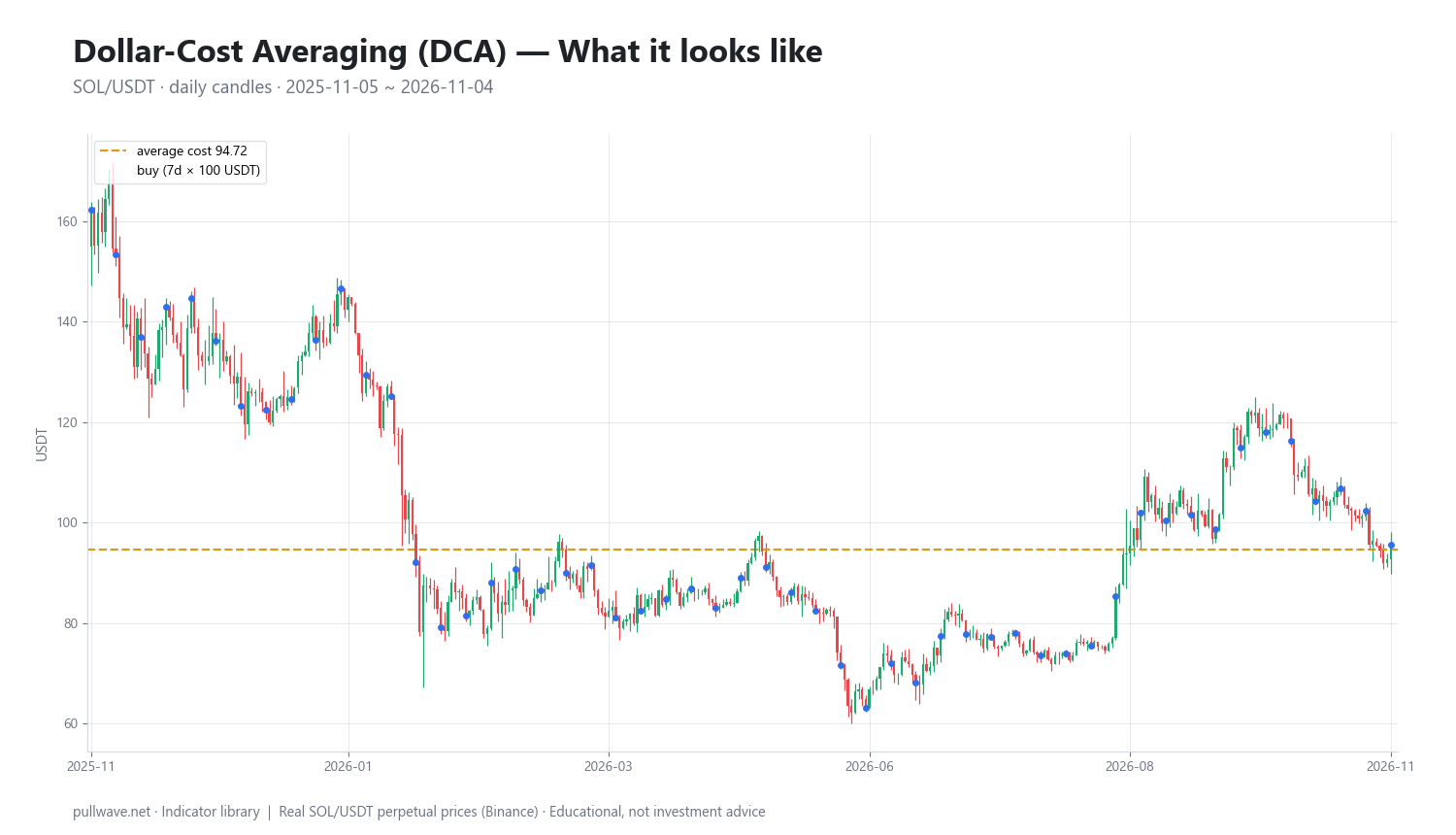
Figure 1 shows the window used throughout this page: SOL/USDT perpetual on Binance, daily candles from 2025-11-05 to 2026-11-04, with the running DCA average cost plotted against price. Notice how the average cost line drops quickly in the first weeks and then flattens, lagging price downward — that is the whole mechanic in one picture.

What is Dollar-Cost Averaging (DCA)?

Dollar-cost averaging is the practice of dividing a total investment into equal cash installments and executing them on a fixed schedule over a period of time, independent of price level, news or indicator readings.

Three elements define any DCA plan:

• Amount per installment — fixed in quote currency (USDT, USD, EUR), not in coins.
• Interval — daily, weekly, bi-weekly, monthly.
• Horizon — how many installments in total, or an open-ended "until further notice" schedule.

The critical distinction: a fixed dollar amount is not the same as a fixed coin amount. Buying 1 SOL per week gives you the arithmetic average of the weekly prices. Buying 100 USDT per week gives you the harmonic average, which is mathematically lower whenever prices vary. That gap is the entire "edge" of DCA, and it is small — it is a cost-averaging effect, not an alpha source.

DCA is also used in the opposite direction. DCA out (or scaling out) means selling a fixed fraction or fixed amount on a schedule to exit a position without having to call the top. The math is symmetric.

The idea behind it (theory and history)

The concept comes from traditional equity investing and predates crypto by decades. It appears in mid-20th-century American investment literature under names such as "dollar averaging" and "constant dollar plan," alongside related formula plans used by investment trusts and accumulation programs.

Benjamin Graham discussed it approvingly in The Intelligent Investor (first edition 1949), presenting it as a disciplined formula for the defensive investor and citing contemporary studies of long-horizon periodic purchasing, including work by Lucile Tomlinson on formula investing. Graham's argument was behavioral as much as mathematical: a mechanical schedule removes the investor's temptation to wait for a better price that may never come.

The theoretical core is simple. With equal cash installments, your average cost is the harmonic mean of the prices paid:

avg_cost = n / (1/P1 + 1/P2 + ... + 1/Pn)

The harmonic mean is always less than or equal to the arithmetic mean, with equality only if every price is identical. More price dispersion means a larger gap. This is why DCA is sometimes described as benefiting from volatility — it does, but only relative to buying the same number of coins each time, not relative to simply buying the low.

There is an important counterpoint that honest teaching requires. Because risk assets have historically spent more time rising than falling, studies on equities (most famously Vanguard's 2012 comparison of lump-sum versus cost averaging) found lump-sum investing produced higher average outcomes roughly two thirds of the time, while DCA produced smaller drawdowns in the bad cases. DCA is a variance-reduction and regret-reduction tool. It is not an expected-return improvement.

How it is calculated

Step by step, in plain words:

1. Fix the installment amount A in quote currency and the interval (for example 100 USDT every 7 days).
2. On each scheduled bar, take the execution price P_i — typically the close, or your actual fill price.
3. Compute the units received: A / P_i. Subtract fees first if you want a realistic cost basis.
4. Keep a running total of units bought and of cash invested.
5. Your average cost is total cash divided by total units.
6. Your position value at any later moment is total units multiplied by the current price.

As a formula:

units_i = A / P_i (per installment) total_units = SUM(units_i) invested = n * A avg_cost = invested / total_units = n / SUM(1/P_i) value_now = total_units * P_now pnl_pct = (P_now / avg_cost - 1) * 100

For the lump-sum comparison you simply buy everything on the first bar:

lump_units = invested / P_first lump_value = lump_units * P_now

If installment sizes vary (some plans scale by signal strength), the general form is avg_cost = SUM(A_i) / SUM(A_i / P_i) — a cash-weighted harmonic mean.

Default settings and variations

There is no canonical "DCA 14" the way there is for RSI. The defaults that circulate come from payroll cycles in traditional finance: monthly investing matched monthly salaries, and the convention stuck. Crypto trades 24/7, so the schedule is a free choice, and the trade-off is between smoothing and friction.

Interval	Installments per year	What it buys you	Main cost
Daily	365	Smoothest average, very low timing variance	Highest fee drag; many tiny fills
Weekly	52	Good smoothing, manageable number of fills	Mild weekday bias (minor)
Bi-weekly	26	Matches many pay cycles	Slightly lumpier entries
Monthly	12	Lowest friction, easiest to maintain	Each buy carries more timing risk

Beyond interval, the common variations are:

• Value averaging — formalized by Michael E. Edleson in his 1991 book Value Averaging. Instead of investing a fixed amount, you target a fixed growth in portfolio value and invest whatever is needed to hit it, buying more after declines and less (or selling) after rallies. Lower average cost in theory, but installment sizes become unpredictable, which is a real constraint for anyone with a fixed budget.
• Filtered or weighted DCA — keep the schedule, but scale the amount by a condition: larger when price is below a long moving average, smaller when it is extended above. This reintroduces discretion and model risk.
• Fixed-horizon entry DCA — split a known sum into, say, eight weekly tranches purely to reduce entry timing risk, then stop. This is the version most relevant to active traders.
• DCA out — mirror schedule for exits.
• Volatility-adjusted spacing — buy on a schedule and add a tranche after each X% decline. Powerful in ranges, dangerous in a sustained downtrend because the installment count is no longer bounded.

For the worked example on this page the settings are deliberately plain: buy 100 USDT every 7 days on the daily close, no fees.

How to read it

A DCA chart has two lines you care about: price, and your running average cost. The relationship between them tells you everything.

• Average cost above price — the position is at an unrealized loss, and each new installment pulls the average cost down. The average cost falls fastest early in the plan, because each installment is large relative to the units already accumulated and the average tracks price closely. Once the position is large, new buys barely move the average, so it becomes sticky and the gap to a still-falling price persists or widens.
• Average cost below price — the position is in profit, and new installments drag the average cost up toward price, diluting the gain slightly.
• Average cost line flattening — the position has grown large relative to each installment. After 50 installments, one more buy closes only about 2% of the distance between the average cost and the new price.
• Distance from average cost — (price / avg_cost - 1) is your position return and is the only number that matters for the plan, not the return since the first buy.

The practical read is not "signal" but "state": am I still accumulating cheaply enough to move my own average, or am I now effectively holding a large position whose fate depends on the trend rather than on my next 100 USDT?

How traders use it

1. Long-horizon accumulation of a core asset. The classic use: fixed amount, fixed interval, large-cap asset, multi-year horizon, no exit date. Works when the asset has a long-run uptrend and you can keep funding installments through drawdowns. Fails when applied to assets that do not recover — a token that trends toward zero produces an ever-falling average cost and an ever-growing loss. DCA assumes survival; it does not create it.

2. Splitting a planned entry (entry smoothing). You want exposure of 5,000 USDT and deploy it in 10 weekly tranches instead of one click. Works when you have no high-conviction timing edge and want to cap the damage from entering the day before a 30% flush. Fails in a market that gaps away immediately — you end up with a higher average cost than lump sum and less exposure during the move. This is the trade you are consciously making: give up some upside to cut the worst case.

3. Scaling out of a position. Sell a fixed amount or fixed percentage per interval into strength. Works in parabolic phases where tops are violent and unforecastable; the schedule guarantees you realize something. Fails in a steady grind higher, where you exit a strong position far too early.

4. Conditional or filtered accumulation. Run the schedule but weight installments by a regime filter — more when price is below the 200-day moving average or when a long-term oscillator is depressed, less when extended. Works in markets with long, deep cycles. Fails when the filter keeps you out for a whole trend, or when "cheap" stays cheap for years. Adding conditions adds the very timing risk DCA was meant to avoid.

A note specific to crypto derivatives: on perpetual futures, "DCA" is often used loosely to mean averaging down on a leveraged losing position. That is a different activity with a different risk profile. Spot DCA has no liquidation price. On leverage, adding to a losing position without adding proportionate margin moves the liquidation price closer to the current price, and the exchange can close the position before any recovery happens. Funding payments also accrue continuously on perps, so holding a leveraged average-down through a long drawdown carries a running cost that spot accumulation does not.

Example on a real SOL chart

The window is SOL/USDT perpetual on Binance, daily timeframe, from 2025-11-05 to 2026-11-04. The rule: buy 100 USDT on the daily close every 7 days, no fees, no filters, no exits.

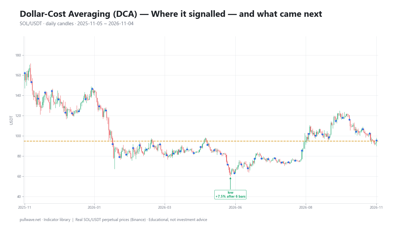
Over the window the plan made 53 buys for a total of 5,300 USDT invested. The first purchase was at 162.28 and the final close was 95.55 — a decline of about 41% in the underlying over the year. The resulting average cost was 94.72, which is just below the final price, so the position finished marginally in profit: 5,346 USDT of value on 5,300 invested, roughly +0.9%.

The lump-sum comparison on the same cash is stark. Deploying all 5,300 USDT at 162.28 on the first bar would have been worth 3,121 USDT at the final close, about −41%. That gap — 5,346 versus 3,121 — is the cost-averaging effect under a falling-then-stabilizing price path. It is also close to the most favorable scenario for DCA, and it would reverse completely in a market that rose steadily from the first bar.

Figure 2 marks the one event flagged in this window: the swing low at 62.16 on 2026-06-06. Six bars later price was +7.45%, and eighteen bars later +9.51% above that level. Installments made near that low bought roughly 1.6 SOL each versus about 0.6 SOL for the opening purchase — the mechanical reason the average cost ended so far below the starting price.

Treat all of this as one illustration on one market over one twelve-month window. A single marked event (1 of 1 resolving higher over both horizons) carries no statistical weight whatsoever; with one observation there is nothing to measure. The outcome here flatters DCA because the path was a long decline into a base. Run the same rule over a window that begins at a cycle low and the lump-sum column wins by a wide margin. Neither result proves anything about the next window.

Common mistakes

• Confusing DCA with averaging down on a leveraged trade. A planned accumulation schedule decided in advance is not the same as adding to a loser because you cannot accept the loss. The second has no horizon, no budget cap, and on futures, a liquidation price.
• Stopping during drawdowns. The installments bought in the worst weeks are the ones that do the work — in the example above, the buys near 62.16 are the reason the average cost reached 94.72. A plan abandoned at the low keeps all the cost and none of the benefit.
• Applying it to assets that can go to zero. DCA has no mechanism for distinguishing a cyclical drawdown from a terminal one. On low-liquidity tokens, a falling average cost is not a bargain, it is a trap.
• No exit plan. Accumulation rules are easy to write; disposal rules are not. Decide in advance whether this is a permanent core position, a multi-year cycle position, or a trade with a target.
• Ignoring fees and spreads. Daily installments on a venue with a fixed minimum fee or wide spreads can give up a meaningful share of the harmonic-mean advantage, which is often only a few percent.
• Over-interpreting backtests. The result of any DCA backtest is almost entirely a function of where the window starts and ends. Shifting the window by three months can flip the conclusion.
• Letting position size drift unmanaged. After enough installments the position may dominate the portfolio. A schedule with no size cap is a concentration plan in disguise.

Combining it with other tools

DCA is a sizing and timing framework, so it layers cleanly on top of analytical tools rather than competing with them.

• Long moving averages (200-day, weekly 50) are the most common overlay: keep the base schedule and increase installment size when price trades below the long average, reduce it when far above. This is a regime filter, not a signal.
• Oscillators on high timeframes — a weekly RSI in deeply oversold territory can mark the stretch of a cycle where extra installments historically landed well. It also stays oversold for long periods in true bear markets, so treat it as a weighting input, not a trigger.
• Volatility measures (ATR, realized volatility) help set the spacing of condition-based tranches. Defining "add after a 15% decline" in ATR multiples adapts the plan to the asset instead of using an arbitrary percentage.
• On-chain valuation metrics such as realized price or MVRV-style ratios are used by longer-horizon accumulators to judge whether the market trades above or below aggregate cost basis. They are slow, cycle-scale inputs, suited to DCA weighting and nothing faster.
• Portfolio rebalancing is the natural companion on the exit side: rather than a calendar sell schedule, trim back to a target allocation whenever the position drifts beyond a band.

The guiding principle: use other tools to adjust how much you commit per installment, and keep the schedule itself mechanical. Once the timing of the installment becomes discretionary, you are back to forecasting.

Frequently asked questions

Q. Is dollar-cost averaging better than lump sum in crypto?

Not on average, but it is better in the bad cases. Because risk assets rise more often than they fall, deploying everything at once has tended to produce higher expected returns over long horizons, while DCA produces shallower worst-case drawdowns and smaller entry-timing regret. In the SOL window on this page DCA finished at 5,346 USDT versus 3,121 for lump sum, but that is one declining-market path, not a general result.

Q. How often should I DCA — daily, weekly or monthly?

Weekly is a common compromise: it smooths entries meaningfully while keeping fee drag and administrative effort low. Daily buying adds very little extra smoothing beyond weekly and multiplies fixed costs; monthly is fine for long horizons but leaves each installment exposed to more short-term timing risk. Choose the interval you can sustain without interruption, because consistency matters more than the exact cadence.

Q. What is the difference between DCA and averaging down?

DCA is a schedule decided before you enter, with a fixed amount, a fixed interval and a defined budget. Averaging down is a reaction to a position that has moved against you, usually with no predetermined limit. The arithmetic of the average cost is identical; the risk management is not, and the distinction matters most on leveraged futures positions.

Q. How do I calculate my average cost in crypto?

Divide the total amount of quote currency you have spent by the total number of coins you received, including fees in the spent amount for a realistic figure. With equal installments this equals the harmonic mean of the purchase prices: n / (1/P1 + ... + 1/Pn). In the example above, 5,300 USDT across 53 buys produced about 55.96 SOL, giving an average cost of 94.72.

Q. Does DCA work in a bear market?

It lowers your average cost during a bear market, which helps when the asset eventually recovers — and does nothing if it does not. The approach depends entirely on the asset surviving and mean-reverting over your horizon, so asset selection and horizon length matter more than the schedule itself. It also requires continuing to fund installments precisely when sentiment is worst, which is the hardest part in practice.

Q. Can you dollar-cost average into leveraged futures positions?

Mechanically yes, but the risk profile is fundamentally different from spot. A leveraged position has a liquidation price, pays or receives funding continuously on perpetuals, and can be closed by the exchange before any recovery, so a plan that "only needs time" may never get it. Anyone applying scheduled entries on futures needs a predefined maximum position size, a maximum number of additions and a stop level set in advance.

Key takeaways

• Dollar-cost averaging invests a fixed cash amount at fixed intervals, so low prices automatically buy more units and the resulting average cost is the harmonic mean of prices paid — always at or below the simple average.
• The concept comes from mid-20th-century equity investing and was popularized by Benjamin Graham in The Intelligent Investor; value averaging, described by Michael Edleson in 1991, is the best-known variation.
• The average cost moves fastest in the first installments and becomes sticky as the position grows, so later buys do little to close the gap to price.
• In the SOL/USDT illustration (53 weekly buys of 100 USDT, 2025-11-05 to 2026-11-04), the average cost settled at 94.72 against a 95.55 close — a favorable path for DCA, and a single window that proves nothing about future outcomes.
• Keep the schedule mechanical, cap total size and horizon in advance, and never let "DCA" become the label for adding to a leveraged losing position.

---

Educational material. Charts use real SOL/USDT perpetual prices; past behaviour does not predict future results. Not investment advice.