At a glance

• BandWidth measures the distance between the Bollinger Bands as a percentage of the middle band, turning band width into a single volatility line.
• A squeeze is an unusually low BandWidth reading, often defined as a multi-month low or as the Bollinger Bands sitting entirely inside the Keltner Channels.
• Compression says a move is likely to expand; it says nothing reliable about direction, and false starts ("head fakes") are common.
• On SOL/USDT 4h in October 2026, 65% of bars qualified as a squeeze and only 4 of 7 breakouts followed through in the signal's own direction.

Bollinger BandWidth is a single line that measures how far apart the Bollinger Bands are, expressed as a percentage of the moving average in the middle. When volatility contracts the line falls; when volatility expands it rises. The "squeeze" is simply the name for an unusually low BandWidth reading — a period when price has gone quiet relative to its own recent history.

Traders care about this because volatility is the one market property that reliably cycles. Quiet periods tend to be followed by active ones and active periods eventually calm down. The squeeze does not tell you which way price will go; it tells you that the current calm is statistically unusual and that the range is more likely to expand than to keep shrinking. That is a narrow piece of information, but a genuinely useful one when you are deciding whether to trade breakouts or fade extremes.

What is Bollinger BandWidth and the Squeeze?

Bollinger Bands plot a moving average with an upper and lower band placed a set number of standard deviations away. Because standard deviation is a volatility measure, the bands widen in turbulent markets and narrow in quiet ones. BandWidth takes that visual property and makes it measurable: it is the gap between the upper and lower band divided by the middle band, usually multiplied by 100.

A squeeze is a low BandWidth reading relative to the same market's recent range of readings. John Bollinger's original definition was mechanical: BandWidth at its lowest value in the last six months. A second widely used definition, popularized later, compares the Bollinger Bands with Keltner Channels — when the bands sit entirely inside the channels, the market is "in squeeze." Both are attempts to answer the same question: is current volatility unusually compressed?

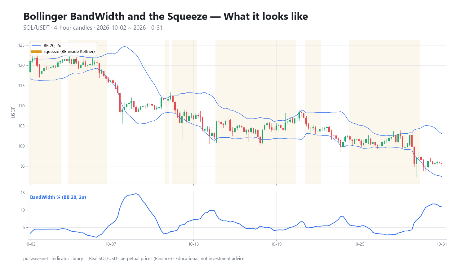
Figure 1 shows SOL/USDT 4h candles with the 20-period, 2-standard-deviation Bollinger Bands drawn on price and the BandWidth line below. Notice how the line collapses toward its lows while the candles cluster into tight sideways ranges, then spikes as soon as a directional move begins.

The idea behind it (theory and history)

Bollinger Bands were developed by John Bollinger in the early 1980s. He wanted bands that adapted to volatility rather than being drawn at a fixed percentage above and below a moving average, which was the common practice at the time. Standard deviation gave him that adaptive quality. Bollinger later introduced two derived indicators — %b, which locates price within the bands, and BandWidth, which measures the bands themselves — and discussed both, along with the squeeze, in his 2001 book Bollinger on Bollinger Bands.

The theory behind the squeeze is volatility clustering: large changes tend to be followed by large changes and small changes by small changes. This is one of the oldest documented statistical features of financial time series and is the basis of the entire GARCH family of volatility models. A squeeze is nothing more than a visual, trader-friendly reading of the low-volatility phase of that cycle.

The Keltner-based variant has its own lineage. Keltner Channels originate with Chester Keltner's 1960 book How to Make Money in Commodities; the modern version built on an exponential moving average and the Average True Range is generally credited to later practitioners, Linda Bradford Raschke among them. Because ATR responds to volatility differently from standard deviation, comparing the two envelopes produces a clean on/off compression signal. John Carter described a version of this approach in Mastering the Trade (2005), which is why many platforms label it a "squeeze" indicator.

One caution Bollinger himself emphasized: the squeeze is frequently followed by a head fake — an initial thrust in one direction that reverses, with the real move going the other way. That is not a flaw in the tool. It is what order flow around a compressed range tends to look like, as stops on both sides get taken before the market commits.

How it is calculated

Step by step, for a 20-period, 2-standard-deviation setting:

1. Compute the middle band: the 20-period simple moving average of closing prices.
2. Compute the standard deviation of those same 20 closes (Bollinger uses the population form, dividing by n).
3. Upper band = middle band + 2 × standard deviation. Lower band = middle band − 2 × standard deviation.
4. BandWidth = (upper band − lower band) ÷ middle band, multiplied by 100 to read it as a percentage.

Because the upper and lower bands are symmetric, step 4 simplifies: the numerator is always 4 standard deviations.

``` MB = SMA(close, 20) SD = StdDev(close, 20) # population UB = MB + 2 * SD LB = MB - 2 * SD BandWidth = 100 * (UB - LB) / MB = 100 * 4 * SD / MB

Keltner-based squeeze state

KC_mid = EMA(close, 20) KC_up = KC_mid + 2 * ATR(10) KC_lo = KC_mid - 2 * ATR(10) squeeze_on = (UB < KC_up) and (LB > KC_lo) ```

Dividing by the middle band is what makes BandWidth comparable across price levels. A $4 band gap means something very different when SOL trades at 240 than at 95; expressing it as a percentage of the average removes that distortion. It does not make readings comparable across different assets or timeframes, which is why most traders judge BandWidth against its own recent percentile rather than against a fixed threshold.

Default settings and variations

Parameter	Common default	Why / when to change
Band period	20	Roughly one month of daily bars in the original stock-market context; long enough to be stable, short enough to adapt
Standard deviations	2	Bollinger's observation that ~2σ contains the large majority of price action for a 20-period average
Average type	SMA	The standard deviation is calculated around the same simple mean, keeping the math internally consistent
Squeeze definition (classic)	BandWidth at a 125-bar low	125 trading days ≈ six months on a daily chart; on crypto 4h charts this is a very long lookback
Squeeze definition (Keltner)	BB 20/2σ vs EMA20 ± 2×ATR10	Gives a binary on/off state instead of requiring a percentile judgment
Keltner ATR multiple	1.5 to 2.0	A lower multiple makes squeezes rarer and more selective

Bollinger suggested that if you shorten the period you should also reduce the multiplier (around 1.9σ for 10 periods) and lengthen it for longer averages (around 2.1σ for 50 periods), so that the proportion of price contained stays similar. Many crypto traders simply keep 20/2 across timeframes and let the chart timeframe do the work.

A useful variation is BandWidth percentile: instead of asking "is BandWidth below 4?", ask "is BandWidth in the bottom 20% of its last 200 readings?" This adapts automatically to assets and regimes that are structurally more or less volatile, and it avoids the trap of carrying a threshold from BTC over to a low-cap altcoin.

How to read it

Read BandWidth as a volatility thermometer, not a price indicator. It has no direction built in: it rises whether price is collapsing or ripping higher.

• Falling BandWidth — the range is contracting. Trend-following entries tend to get chopped; mean-reversion inside the range tends to work better.
• BandWidth at a local low (squeeze) — compression is at an extreme. The probability of a range expansion in the near future is elevated. Direction unknown.
• BandWidth turning up sharply off a low — expansion has begun. This is the moment the squeeze "fires."
• BandWidth very high (Bollinger called the extreme a "bulge") — the move is already mature. Entering breakouts here means paying for volatility you have already missed, and stops have to be wide.

The practical sequence is: compression → expansion → trend or failure → compression again. Your job is to know which phase you are in before choosing a tactic.

How traders use it

1. Breakout preparation. When BandWidth sits near the bottom of its range, traders mark the high and low of the compression range and plan for an expansion through either side. Works when the squeeze is long, tight and follows a clear trend — the pause is often continuation. Fails in persistently rangebound markets, where each "breakout" reverses within a few bars. The head-fake risk is highest when the squeeze forms at the middle of a wider range rather than at its edge.

2. Position sizing and stop placement. Because BandWidth is proportional to standard deviation, it is a direct input to risk. In a squeeze, the same dollar risk allows a much tighter stop, and the same stop distance allows a larger position. Works as a risk-management discipline, because it forces you to price the current range before choosing size. Fails as a signal if you size up during compression and forget that volatility — and therefore liquidation distance on leveraged positions — can triple within a few bars.

3. Regime filter for other indicators. Oscillators like RSI or Stochastics behave well in low-BandWidth ranges and generate relentless false signals once a trend expands. Trend tools do the opposite. Using BandWidth percentile as a switch between the two toolsets is one of its most durable applications. Fails when regime changes happen mid-trade; the filter lags.

4. Exhaustion awareness. A BandWidth spike to multi-month highs after a long directional run signals that volatility is stretched, which often precedes consolidation or a sharp retracement. Works as a reason to tighten management on an existing position. Fails badly as a reversal signal on its own — parabolic markets can keep expanding far longer than seems reasonable.

Example on a real SOL chart

The window below is SOL/USDT perpetual futures, 4-hour bars, from 2026-10-02 to 2026-10-31, using Bollinger 20/2σ against a Keltner reference of EMA20 ± 2×ATR10. This is one market over one month. It is an illustration of how the readings behave, not evidence that the technique works.

Over the window, BandWidth ranged from a low of 2.13 to a high of 14.73, closing the period at 10.90. The compression was unusually persistent: 65.0% of all bars in the window met the Keltner-based squeeze condition. Seven squeeze-to-breakout events were recorded. Forward performance was measured after 6 bars (one day) and 18 bars (three days).

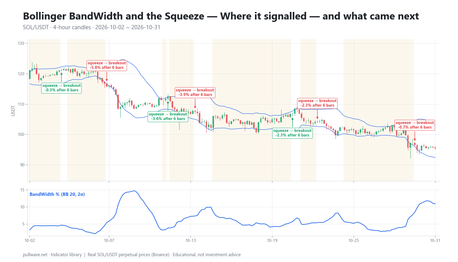
Figure 2 marks each of the seven events on the same chart and labels the percentage move that followed over both horizons.

Date (UTC)	Price at signal	After 6 bars	After 18 bars
2026-10-04 08:00	121.17	−0.35%	−3.20%
2026-10-07 16:00	115.81	−5.81%	−4.65%
2026-10-12 04:00	112.54	−3.58%	−8.28%
2026-10-14 04:00	107.44	−3.93%	−2.23%
2026-10-21 08:00	106.82	−2.27%	−5.01%
2026-10-23 04:00	104.25	−2.30%	−3.42%
2026-10-30 08:00	96.53	−0.73%	−1.13%

Two things stand out, and neither is flattering in a simple way. First, every single forward return in the table is negative. That is a property of the month, not of the indicator: SOL fell from 121.17 at the first event to a last close of 95.44, roughly a fifth of its value, so any signal in this window was measured inside a downtrend. Second, when each breakout is scored against its own direction — did price continue the way the bands broke? — only 4 of 7 followed through over the measurement horizon. Three breakouts resolved against themselves, which is exactly the head-fake behavior Bollinger warned about.

The useful lesson here is not a win rate. It is that a market can spend two-thirds of a month in compression and still trend steadily lower, and that squeeze signals during a downtrend were far kinder to short-side continuation than to anyone fading the move. With a sample of seven, nothing here is statistically meaningful. Treat it as a reading exercise.

Common mistakes

• Treating the squeeze as directional. It is a volatility statement. Any direction must come from structure, trend context or another tool.
• Using a fixed BandWidth threshold across assets. A reading of 3 is extreme compression for BTC on a daily chart and ordinary for a thin altcoin on 5-minute bars. Use percentile ranks.
• Ignoring the head fake. Planning only for a clean break in one direction leaves you with no plan when the first thrust reverses. Many traders explicitly allow for the initial move to fail.
• Sizing up because stops are tight. Compression makes stops tight and tempts leverage. On perpetual futures, an expansion of 3–5x in BandWidth within a day can put a liquidation price that looked safe directly in the path of a normal wick.
• Chasing after the expansion. Entering when BandWidth is already near its high means buying volatility at its most expensive, with the worst reward-to-risk of the cycle.
• Over-reading very short timeframes. Crypto trades 24/7, and the 1- and 5-minute charts produce squeezes during low-liquidity hours that mean nothing more than "nobody is awake."

Combining it with other tools

BandWidth answers "how much movement?" so it pairs naturally with tools that answer "which way?" Horizontal support and resistance is the simplest and often the best partner: a squeeze that forms directly beneath a well-tested level gives the breakout a reason to exist. Trendlines and the slope of a longer moving average serve the same purpose.

%b, Bollinger's companion indicator, is the natural complement. BandWidth tells you the bands are tight; %b tells you where price sits inside them. A squeeze that resolves with %b pushing above 1 is a different event from one where price stalls at the middle band.

Volume and, for perpetuals, open interest add a confirmation layer. An expansion backed by rising volume and growing open interest reflects new positioning; one on fading volume more often reflects a stop run. Funding rates can add context too — a breakout into heavily one-sided funding is more vulnerable to a sharp unwind.

Finally, ATR deserves a mention as a sibling rather than a substitute. ATR measures absolute range including gaps and wicks; standard deviation measures dispersion of closes. They often agree, and when they disagree — ATR high, BandWidth low — it usually means wide wicks around a flat close structure, which is worth knowing before you assume the market is quiet.

Frequently asked questions

Q. What is a Bollinger Band squeeze?

A Bollinger Band squeeze is a period when the Bollinger Bands narrow to an unusually small width, indicating that volatility has contracted well below its recent norm. It is commonly defined either as BandWidth hitting a multi-month low or as the Bollinger Bands closing entirely inside the Keltner Channels. The squeeze suggests a range expansion is more likely than continued quiet, but it gives no information about direction.

Q. What is the best Bollinger BandWidth setting for crypto?

Most traders keep Bollinger's defaults of a 20-period simple moving average with 2 standard deviations, because the formula was designed around that pairing. What matters more in crypto is how you define "low" — using a rolling percentile (for example, the bottom 20% of the last 200 readings) adapts to each asset instead of importing a fixed threshold. On 4h and daily charts the readings are far more stable than on sub-hourly charts.

Q. Does a squeeze predict the direction of the breakout?

No. BandWidth is derived from standard deviation, which is direction-neutral by construction, so a squeeze can resolve either way. John Bollinger specifically described the "head fake," where the first move out of a squeeze reverses and the real move goes the other way. Direction has to come from trend context, market structure or a separate indicator.

Q. How long does a Bollinger Band squeeze last?

There is no fixed duration — squeezes can last a few bars or persist for weeks. In the SOL 4h example above, 65% of bars in a one-month window met the squeeze condition, which shows how long compression can drag on. As a rough guide, longer and tighter squeezes tend to precede larger expansions, but this is a tendency, not a rule.

Q. What is the difference between BandWidth and %b?

BandWidth measures the width of the bands relative to the middle band and describes volatility. %b measures where the current price sits between the lower band (0) and the upper band (1) and describes position. They are complementary: one tells you how big the envelope is, the other tells you where you are inside it.

Q. Is the squeeze useful on leveraged perpetual futures?

It can be, mainly as a risk-management input. Low BandWidth means current volatility understates near-term risk, so stop distances and liquidation buffers calculated during a squeeze may be far too tight once the range expands. Many traders deliberately reduce leverage into compression rather than increase it.

Key takeaways

• BandWidth = (upper band − lower band) ÷ middle band × 100, which simplifies to 4 standard deviations as a percentage of the 20-period average.
• A squeeze is an extreme low in BandWidth, defined either by a multi-month low or by the Bollinger Bands sitting inside Keltner Channels (EMA20 ± 2×ATR10 is a common reference).
• Compression forecasts expansion, never direction; head fakes out of squeezes are normal and should be planned for.
• Judge BandWidth by percentile against its own history rather than by a fixed number copied between assets or timeframes.
• In the October 2026 SOL 4h window, 65% of bars were in squeeze, BandWidth ran from 2.13 to 14.73, and only 4 of 7 breakouts followed through — a reminder that one window on one market proves nothing either way.

---

Educational material. Charts use real SOL/USDT perpetual prices; past behaviour does not predict future results. Not investment advice.